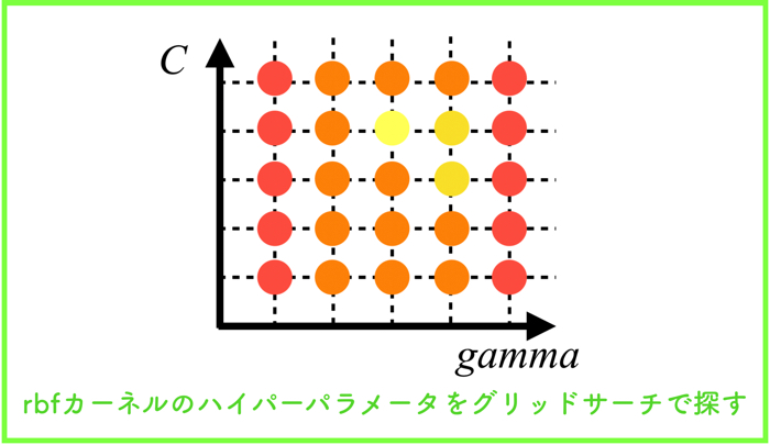
- サポートベクターマシンで用いるRBFカーネルのハイパーパラメータ\(\gamma, C\)について
- for文でグリッドサーチをしてみる.
- ベイズ最適化による探索も試す!
こんにちは.けんゆー(@kenyu0501_)です.
前回の続きなのですが,今回はrbfカーネル(ガウスカーネル)のハイパーパラメータをグリッドサーチで探索したいと思います.
(前回:各種カーネル関数を使ってサポートベクターマシンを実装する)
ハイパーパラメータとは,SVMを設計する人が経験的かつ独自に決めるべき定数です.
扱う系によって最適な値が変わるので,分類器を構築する前に,どの程度の値が良いのかざっと調べるべき必要があります.
これらは,ヒューリスティックでありますが,いくつか求め方もあります.
ヒューリスティックとは,必ずしも正しい答えを導けるわけではないけど,ある程度のレベルで正解に近い解を得られることだよ!
RBFカーネルのハイパーパラメータ
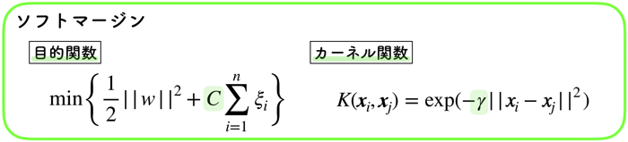
RBFのハイパーパラメータは以上の2つです.
- コスト関数の \(C\)
- カーネル関数の \(\gamma\)
これらは,デフォルトで回すと以下のような値を持っています.
SVC(C=1.0, cache_size=200, class_weight=None, coef0=0.0,
  decision_function_shape='ovr', degree=3, gamma='auto_deprecated',
  kernel='rbf', max_iter=-1, probability=False, random_state=None,
  shrinking=True, tol=0.001, verbose=False)
\(\gamma\) は’auto_deprecated’,Cは1.0を持っていますね.
これらの値をグリッドサーチにて探していきましょう!
グリッドサーチ(GS)とは!?
グリッドサーチ,名前はかっこいいですが,単なるしらみ潰し探索です.
ちょっとずつパラメータの値を変えて,汎化性能を調べていくという作業になります.
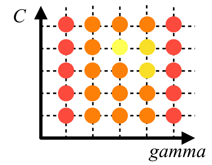
具体的には,横軸に\(\gamma\),縦軸に\(C\)をとって,各軸のグリッド線が交差する箇所のパラメータを使って汎化性能を確認する!というかなりシンプルなものです.
pythonだとライブラリが出ていますが,シンプルなものなので,for文で書きました.
ちなみに,sklearnから,GridSearchCVというライブラリが出ているので,こちらを使っても大丈夫です!
GSの結果とそのハイパーパラメータを使ったSVM
<GSの条件>
- 各パラメータ\(\gamma,C\),0.01から10まで,100分割をした.
- 100×100=10000回の総当たり計算をした
- 特に,交差検証などは行っていない.
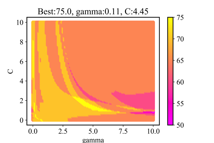
グリッドサーチ(GS)の結果を上に示します.
10000回の総当たり計算を行いました.
成績の良いものを黄色,成績の悪いものをピンクで示しました.
この時の成績とは,ハイパーパラメータを使ったSVMの汎化性能だよ!教師データ(80%)で分離境界面を作って,残りの20%でテストした結果だよ!
GSを行ったハイパーパラメータ\(\gamma,C\)はそれぞれ,0.1と4.4でした.
そのパラメータを使った結果を以下に示します.
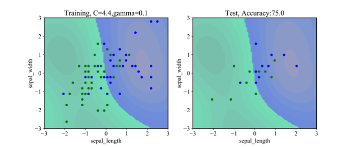
左側が,トレーニングデータ(80%)を使ったもので,右側がテストデータ(20%)です.
データ自体が,凄く入り組んでいるので,あまりrbfカーネルの良さが生かされていないような気もしますが,,,笑
プログラムについて
#!/usr/bin/env python3
# -*- coding: utf-8 -*-
"""
Created on Sat Aug 24 11:33:41 2019

@author: ueharakenyuu
"""
import numpy as np
import matplotlib.pyplot as plt
import pandas as pd
from sklearn.datasets import load_iris
from sklearn.preprocessing import StandardScaler
from sklearn.model_selection import train_test_split
from sklearn.svm import SVC

#------データの読み込みと使うデータの選択-----------#
iris_dataset = load_iris()
X = iris_dataset.data
y = iris_dataset.target

X_sl = np.vstack((X[:, :1]))
X_sw = np.vstack((X[:, 1:2]))
X_pl = np.vstack((X[:, 2:3]))
X_pw = np.vstack((X[:, 3:4]))

X = np.hstack((X_sl,X_sw))

X = X[y!=0]
y = y[y!=0]
scaler = StandardScaler()
X = scaler.fit_transform(X)

X_train, X_test, y_train, y_test = train_test_split(X, y, test_size = 0.2,random_state = 0)
#------データの読み込みと使うデータの選択-----------#

#------グリッドサーチ-----------#
best_score = float(0.0)
best_param_gamma = 0.0
best_param_C = 0.0

scores = pd.DataFrame()
for gamma in np.linspace(0.01, 10, 100):
    for C in np.linspace(0.01, 10, 100):
        svm = SVC(kernel = 'rbf', gamma=gamma, C=C)
        svm.fit(X_train, y_train)
        scores = scores.append(
                {
                    'gamma': gamma,
                    'C': C,
                    'accuracy': svm.score(X_test, y_test)
                },
                ignore_index=True)

        if best_score < svm.score(X_test, y_test):
            best_score = svm.score(X_test, y_test)
            best_param_gamma = gamma
            best_param_C = C

print("ベストスコア:", round(best_score,2))
print('g:%s c:%s' %(round(best_param_gamma,2),round(best_param_C,2)))

fig, ax = plt.subplots()
ax.set_xlabel('gamma')
ax.set_ylabel('C')
ax = ax.scatter(scores.gamma, scores.C, c=100.0*scores.accuracy, cmap='spring')
fig.colorbar(ax)
plt.title('Best:{}, gamma:{}, C:{}'.format(100*round(best_score,3), round(best_param_gamma,2),round(best_param_C,2)))
fig.savefig('output_gs.png',dpi=900)
#------グリッドサーチ-----------#

#------グリッドサーチで求めた最適なパラメータでSVMを回す-----------#
gamma = best_param_gamma
C = best_param_C

svm = SVC(kernel = 'rbf', gamma=gamma, C=C)

svm.fit(X_train, y_train)
R = svm.predict(X_test)
total = len(X_test)
success = sum(R == y_test)
print("Accuracy is:{}".format(100*success/total))
#------グリッドサーチで求めた最適なパラメータでSVMを回す-----------#

#----------グラフ描写用の関数---------------#
def plot_decision_function(model):
    _x0 = np.linspace(-3.0, 3.0, 100)
    _x1 = np.linspace(-3.0, 3.0, 100)
    x0, x1 = np.meshgrid(_x0, _x1)
    X = np.c_[x0.ravel(), x1.ravel()]
    y_pred = model.predict(X).reshape(x0.shape)
    y_decision = model.decision_function(X).reshape(x0.shape)
    plt.contourf(x0, x1, y_pred, cmap='winter_r', alpha=0.4)
    plt.contourf(x0, x1, y_decision,levels=10, alpha=0.2)

def plot_dataset(X,y):
    plt.plot(X[:, 0][y==2], X[:, 1][y==2], "bo", ms=5)
    plt.plot(X[:, 0][y==1], X[:, 1][y==1], "go", ms=5)
    plt.xlabel("sepal_length")
    plt.ylabel("sepal_width")
#---------------------------------------#

#--グラフを描写するor保存する(1行2列で)------#

plt.figure(figsize=(12,5))
plt.subplot(121)
plot_decision_function(svm)
plot_dataset(X_train,y_train)
plt.title('Training, C={:.1f},gamma={:.1f}'.format(C,gamma))

plt.subplot(122)
plot_decision_function(svm)
plot_dataset(X_test,y_test)
plt.title('Test, Accuracy:{:.1f}'.format(100.0*success/total))
plt.savefig('svm_output.png',dpi=900)
#plt.show()
#--------------------------------------#
グリッドサーチは,for文を2回,くるくる回しています.
for文を抜けた後には,その中で最も良かったベストなハイパーパラメータを使って,もう一度SVMを回してます.
おまけ:ベイズ最適化でハイパーパラメータを探索
グリッドサーチで探索しても良いですが,網羅的に探索する総当たり計算はあまり芸がないようにも思います.
そのため,今回はおまけとして,ベイズ最適化を使ったハイパーパラメータの探索も試みました.
以下に結果を示します.
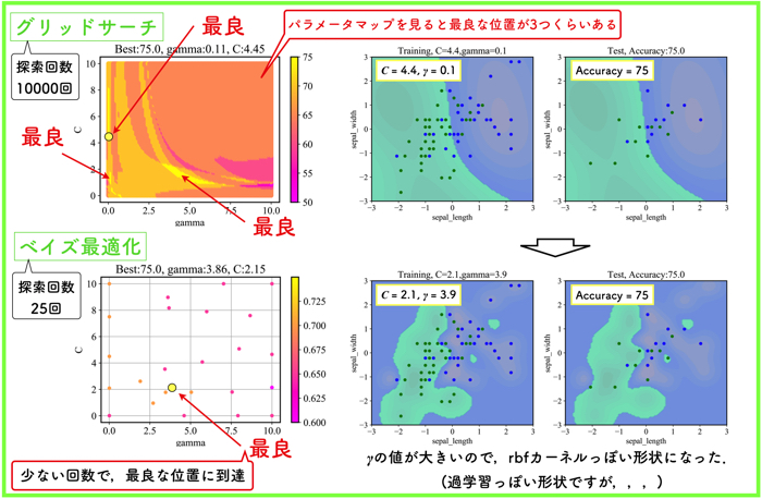
グリッドサーチで探した範囲において,ベイズ最適化を試みたので,最良点が探しだせていることがわかります.
ただ,ハイパーパラメータの値自体は異なるので,分離平面が全く異なるという結果になりました.
(グリッドサーチの探索するサンプリング間隔にもよりますが,だいぶ細かくとりました)
\(\gamma\) の値が大きくなると,境界がものすごく複雑になることが確認できるね!教師データを使ったデータセットには上手く適合しそうだけど,未知のデータには汎化誤差が出てくるような気もするね!今回はたまたま上手くいっているけど.
\(\gamma\) の値は過学習を抑制するためにも重要なパラメータであることが分かるね!
交差検証を行っていないので,信憑性に関しては低いですが,プログラムとしては機能しているようです.
また,以下の表にベイズ最適化の過程において,選択された値を示します.
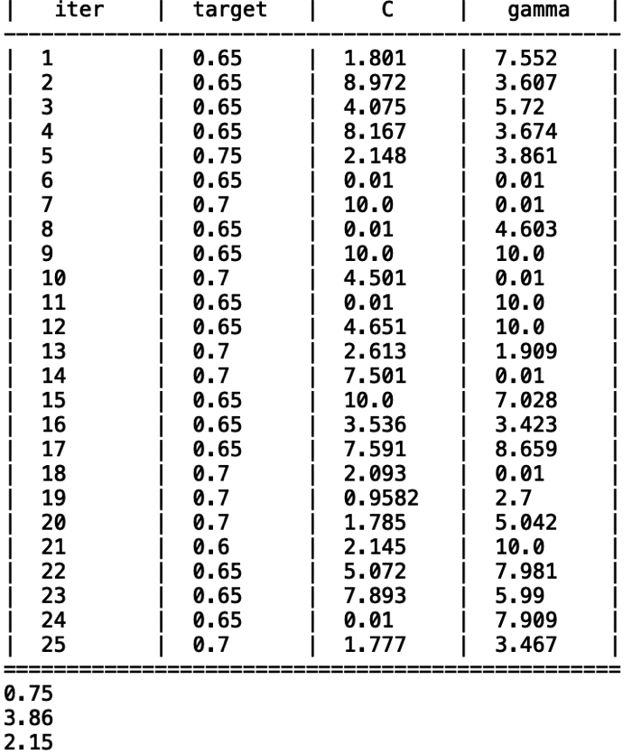
初期値が初めの5つで,20回(iteration),計算しました.
20回でも最良(汎化性能が高い点)を探索できているようです.
プログラムも載せておきますね!
ベイズ最適化によるプログラムについて
#!/usr/bin/env python3
# -*- coding: utf-8 -*-
"""
Created on Sat Aug 24 11:33:41 2019

@author: ueharakenyuu
"""

import numpy as np
import matplotlib.pyplot as plt

from sklearn.datasets import load_iris
from sklearn.preprocessing import StandardScaler
from sklearn.model_selection import train_test_split

from sklearn.svm import SVC

from bayes_opt import BayesianOptimization

#------データの読み込みと使うデータの選択-----------#
iris_dataset = load_iris()

X = iris_dataset.data
y = iris_dataset.target

X_sl = np.vstack((X[:, :1]))
X_sw = np.vstack((X[:, 1:2]))
X_pl = np.vstack((X[:, 2:3]))
X_pw = np.vstack((X[:, 3:4]))

X = np.hstack((X_sl,X_sw))

X = X[y!=0]
y = y[y!=0]

scaler = StandardScaler()
X = scaler.fit_transform(X)

X_train, X_test, y_train, y_test = train_test_split(X, y, test_size = 0.2,random_state = 0)
#------データの読み込みと使うデータの選択-----------#

#------ベイズ最適化-----------#
def f(gamma, C):
    svm = SVC(kernel = 'rbf', gamma=gamma, C=C)
    svm.fit(X_train, y_train)
    return  svm.score(X_test, y_test)

pbounds = {
    'C': (0.01, 10),
    'gamma': (0.01, 10)
}
bo = BayesianOptimization(f=f, pbounds=pbounds)

bo.maximize(init_points=5, n_iter=20, acq='ucb')

print(round(bo.max['target'],3))
print(round(bo.max['params']['gamma'],2))
print(round(bo.max['params']['C'],2))

gamma = [p['params']['gamma'] for p in bo.res]
C = [p['params']['C'] for p in bo.res]
score = [p['target'] for p in bo.res]


sc = plt.scatter(gamma, C, c=score, s=20, zorder=10, cmap='spring')
plt.colorbar(sc)

plt.xlabel('gamma')
plt.ylabel('C')
plt.grid()
plt.title('Best:{}, gamma:{}, C:{}'.format(100*round(bo.max['target'],3), round(bo.max['params']['gamma'],2),round(bo.max['params']['C'],2) ) )
plt.savefig('bayes_opt.png',dpi=900)
#------ベイズ最適化-----------#
#------BOで求めた最適なパラメータでSVMを回す-----------#
gamma = bo.max['params']['gamma']
C = bo.max['params']['C']

svm = SVC(kernel = 'rbf', gamma=gamma, C=C)

svm.fit(X_train, y_train)
R = svm.predict(X_test)
total = len(X_test)
success = sum(R == y_test)
print("Accuracy is:{}".format(100*success/total))
#------BOで求めた最適なパラメータでSVMを回す-----------#

#----------グラフ描写用の関数---------------#
def plot_decision_function(model):
    _x0 = np.linspace(-3.0, 3.0, 100)
    _x1 = np.linspace(-3.0, 3.0, 100)
    x0, x1 = np.meshgrid(_x0, _x1)
    X = np.c_[x0.ravel(), x1.ravel()]
    y_pred = model.predict(X).reshape(x0.shape)
    y_decision = model.decision_function(X).reshape(x0.shape)
    plt.contourf(x0, x1, y_pred, cmap='winter_r', alpha=0.4)
    plt.contourf(x0, x1, y_decision,levels=10, alpha=0.2)

def plot_dataset(X,y):
    plt.plot(X[:, 0][y==2], X[:, 1][y==2], "bo", ms=5)
    plt.plot(X[:, 0][y==1], X[:, 1][y==1], "go", ms=5)
    plt.xlabel("sepal_length")
    plt.ylabel("sepal_width")
#---------------------------------------#

#--グラフを描写するor保存する(1行2列で)------#

plt.figure(figsize=(12,5))
plt.subplot(121)
plot_decision_function(svm)
plot_dataset(X_train,y_train)
plt.title('Training, C={:.1f},gamma={:.1f}'.format(C,gamma))

plt.subplot(122)
plot_decision_function(svm)
plot_dataset(X_test,y_test)
plt.title('Test, Accuracy:{:.1f}'.format(100.0*success/total))
plt.savefig('svm_output.png',dpi=900)
#plt.show()
#--------------------------------------#
また,今度,ベイズ最適化については詳細な記事を書きます!