2019年になりましたね!
2018年は12月28日に研究納めをしましたが,2019年は1月1日から研究を開始していきます.
ということで,現在やっているパラメタ同定奮闘記の続きを書いていきます.
(完全なる自分用の研究アーカイブなので,雑に書いてますので読みにくいと思います...)
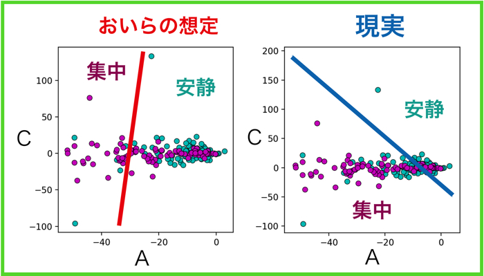
何をやっているのかというと,脳波の状態(集中とか安静とか)を解析するための数学モデルを作っています.
具体的には,内側のモデルパラメータを逆問題で同定して,パラメータの値によって複雑な脳波の状態が評価できないか?
ということをしているのですが,逆問題を解くための条件設定が色々と難しいので四苦八苦してるという状態です笑
前回の内容の復習
以前の記事はこちら
この記事は,脳波からヒトの状態推定を可能にするモデルをどうにか作りたくて獅子奮闘している研究アーカイブ(自分用…
前回は,
・解析窓ごとにFFT
・ピークを一つ決める
・検討する周波数帯域をあらかじめ,ピークが属する帯域でIFFT
・IFFTで得た1秒間の時系列波形を用いてパラメタ同定
という流れでしたね.
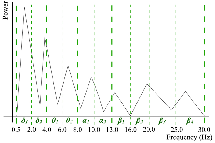
しかし,前回はFFTを行う時に,解析窓の幅が狭かったので周波数分解能はかなり低くて1Hz程度なのがちょっと問題でした.
周波数分解能というのは,以下を見てください!
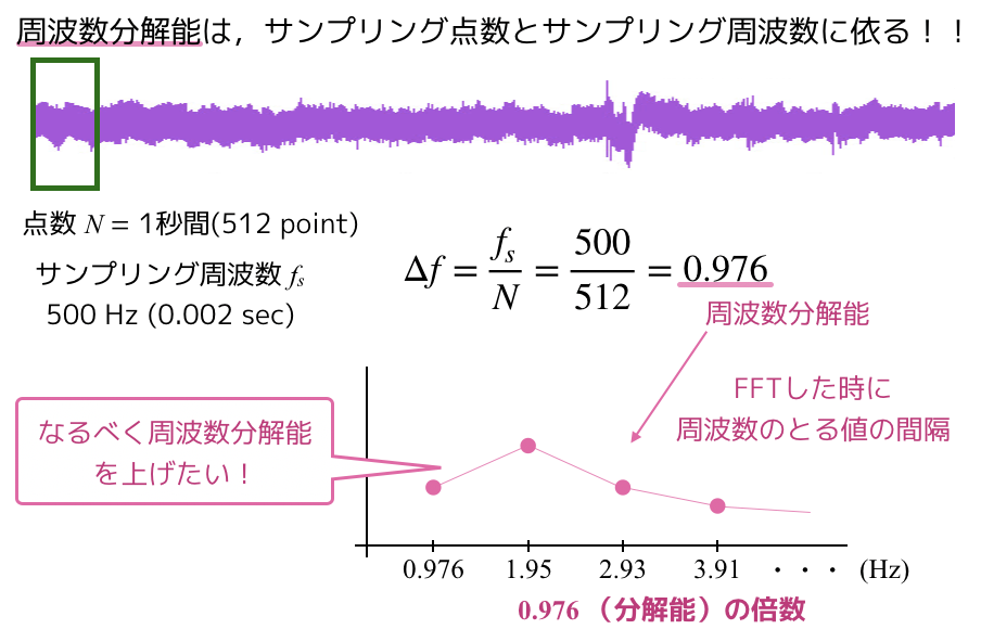
現在の周波数分解能は,0.976Hz,約1Hzです.
そう,生波形の周波数解析をして,どのくらいの周波数が含まれているのかを確認する時に,約1Hzの分解能しか調べることができません.
ちょっと生体信号を扱う上では不便ですよね.もう少し細かく0.25Hz毎とかで調べたいわけですよ.
そのため,どういう対策をするかというと,
- 解析窓の幅をもっと長くする
- サンプリング周波数をもっと短くする
の二つの方法が考えられます.
サンプリング周波数の間隔は,脳波データを取得する実験装置の方で設定する必要があるので,データを取った今,この間隔を短くするのはちょっと無理です.
(厳密には補間することが可能ですが,,,)
そこで,実験データの構造を壊さず解析するために,解析窓の幅を増やすということをします.
今回の内容について
よって今回は以下のような修正を行います.
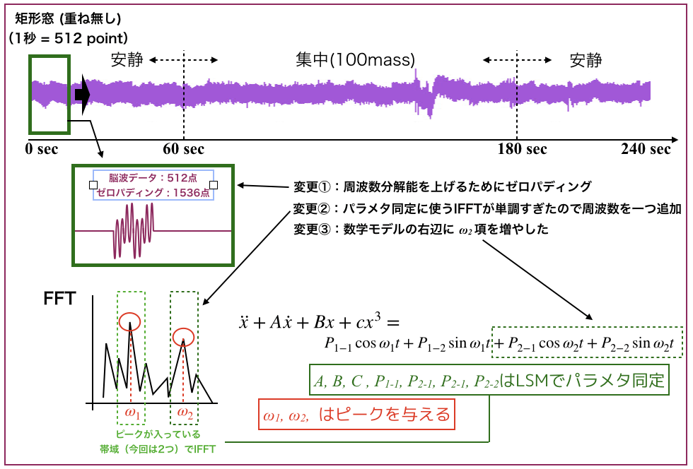
変更箇所は3箇所です.
- 周波数分解能を上げるためにゼロパディングをする
- パラメタ同定に使うIFFTが単純すぎたので周波数を一つ追加
- 数学モデルの右辺にωの項をもう一つ追加
です.
1秒毎に解析するこだわりは特にないのですが,ゼロパディングをして周波数成分の量を破壊せずに分解能を上げるということをしました.
サンプリング点数の量を稼ぐために,変動しない値(0)を解析窓に挿入する方法です.
(今回は解析窓毎の波形の平均値を3秒分挿入してます)
解析結果
パラメータ同定結果
早速そういうふうな改良でパラメタ同定したものを以下に示します.
また,先に結果から言っておくと,0.5Hz〜を含めた周波数解析結果は,解析窓毎の周波数が圧倒的に低周波数側に寄ってしまったので,以下二つの条件でやります.
周波数条件①:0.5 – 30.0 Hz
周波数条件②:4.0 – 30.0 Hz
デルタ帯域(0.5 – 4.0 Hz)が入っているかどうかの違いです.
以下は周波数条件①
上のグラフから生脳波データ,
その下のグラフは解析窓のデータ+平均値パディング(ゼロパディング)
その下は周波数解析の結果.
下の3×3の小さめのグラフはパラメタです.
見にくくてごめんなさい.
 以下は周波数条件②
いい感じに,周波数ピークの獲得がされていて,集中状態や安静状態が判別できそう...?です笑
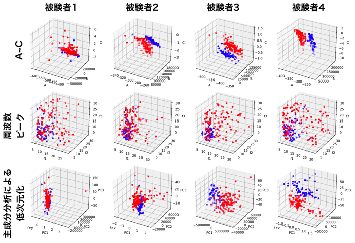
いちよう,前回の記事を見てもらったら話が早いのですが,被験者は4人いるので,それぞれやって,パラメタの相関を調べました.
(最小二乗法によるパラメータ同定奮闘記2)
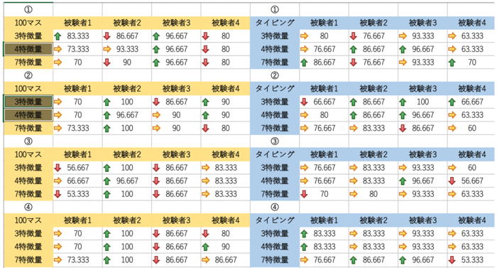
各被験者,各パラメタの相関
周波数条件① 0.5 – 30 Hz
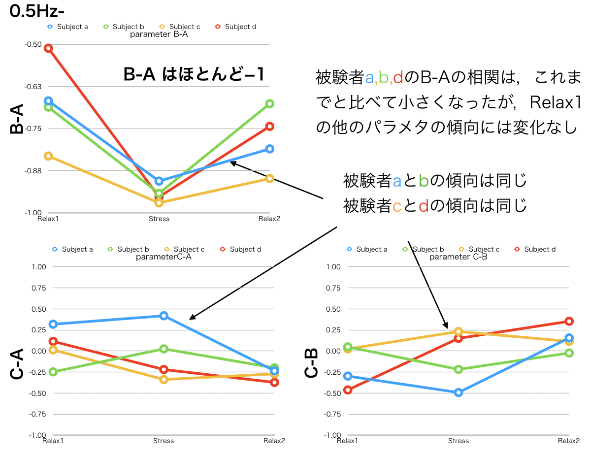
以下,観測結果をまとめました
・ゼロパディングとω2 を追加 → リラックス状態のA-Bの相関が小さくなってきた.
・しかし,まだC-B間の傾向ははっきりしたものはない.
・集中すると,A-Bの相関は -1へ近づくことが分かった.
・ただ,やっぱり低周波帯域(デルタ)の影響がかなり大きいので,デルタを抜いた方が良いのかもしれない.
周波数条件② 4.0 – 30 Hz
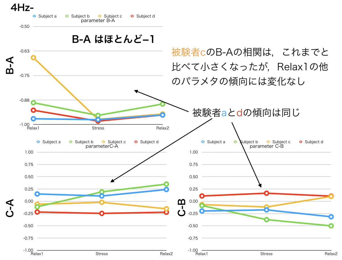
以下に観測結果をまとめます.
・デルタ帯域を抜いた場合でパラメタ同定を行うと,これまでの被験者ごとの傾向が全く異なる.
・デルタ帯域を抜いて,かなり傾向が変わるので,この帯域を入れるかどうかがパラメタ同定にかなり影響する.
・モデルの改良(vanderPol導入 or 右辺の項)や帯域の制限(アルファのみ?)などを色々と調べる必要がある.
プログラムについて
ゼロパディングを入れて,アニメーション出力までやってくれるPythonプログラムです.
1 2 3 4 5 6 7 8 9 10 11 12 13 14 15 16 17 18 19 20 21 22 23 24 25 26 27 28 29 30 31 32 33 34 35 36 37 38 39 40 41 42 43 44 45 46 47 48 49 50 51 52 53 54 55 56 57 58 59 60 61 62 63 64 65 66 67 68 69 70 71 72 73 74 75 76 77 78 79 80 81 82 83 84 85 86 87 88 89 90 91 92 93 94 95 96 97 98 99 100 101 102 103 104 105 106 107 108 109 110 111 112 113 114 115 116 117 118 119 120 121 122 123 124 125 126 127 128 129 130 131 132 133 134 135 136 137 138 139 140 141 142 143 144 145 146 147 148 149 150 151 152 153 154 155 156 157 158 159 160 161 162 163 164 165 166 167 168 169 170 171 172 173 174 175 176 177 178 179 180 181 182 183 184 185 186 187 188 189 190 191 192 193 194 195 196 197 198 199 200 201 202 203 204 205 206 207 208 209 210 211 212 213 214 215 216 217 218 219 220 221 222 223 224 225 226 227 228 229 230 231 232 233 234 235 236 237 238 239 240 241 242 243 244 245 246 247 248 249 250 251 252 253 254 255 256 257 258 259 260 261 262 263 264 265 266 267 268 269 270 271 272 273 274 275 276 277 278 279 280 281 282 283 284 285 286 287 288 289 290 291 292 293 294 295 296 297 298 299 300 301 302 303 304 305 306 307 308 309 310 311 312 313 314 315 316 317 318 319 320 321 322 323 324 325 326 327 328 329 330 331 332 333 334 335 336 337 338 339 340 341 342 343 344 345 346 347 348 349 350 351 352 353 354 355 356 357 358 359 360 361 362 363 364 365 366 367 368 369 370 371 372 373 374 375 376 377 378 379 380 381 382 383 384 385 386 387 388 389 390 391 392 393 394 395 | # -*- coding: utf-8 -*- import csv import scipy.signal as sps from scipy.optimize import leastsq import numpy as np import matplotlib.pyplot as plt import matplotlib.animation as animation import matplotlib.patches as patches from time import sleep frame = 241 #定数宣言 N = 512 # サンプル数 dt = 0.002 # サンプリング間隔 p_max = 30.0 p_min = 0.5 #p_band = 1.00000 delta_bound, theta_min, theta_bound, alpha_min, alpha_bound, beta_min, beta_bound1, beta_bound2, beta_bound3 = 2.0, 4.0, 6.0, 8.0, 10.0, 13.0, 16.0, 20.0, 25.0 #fftゼロぱっディング用 n_b = 512 n_a = 1024 #ファイル名宣言 inputData = 'exp.txt' outputPara = 'parameters_d_100mass_0.5Hz.txt' outputIFFT = 'ifft_d_100mass_0.5Hz.txt' outputMovie = 'result_d_0.5Hz.mp4' rowN = 4 #配列用意 x_exp = list() x_ifft = np.empty((2,0)) t = list() xd = list() xdd = list() w = list() p = list() x_ifft_s = list() x_exp_s = list() t_s = list() Result = list() F2 = list() freq = list() Power = list() x_exp_ss = list() x_ifft_ss = list() timecount = 1 #global #const. t_max = 250 t_min = 0 window = N*dt timestep = 0 #timestep def det_band(frequencies): global p_min, p_max, delta_bound, theta_min, theta_bound, alpha_min, alpha_bound, beta_min, beta_bound1, beta_bound2, beta_bound3 f_max = list() f_min = list() k = 0 for frequency in frequencies: if((p_min <= frequency)&(frequency < delta_bound)): f_min.append(p_min) f_max.append(delta_bound) elif((delta_bound <= frequency)&(frequency < theta_min)): f_min.append(delta_bound) f_max.append(theta_min) elif((theta_min <= frequency)&(frequency < theta_bound)): f_min.append(theta_min) f_max.append(theta_bound) elif((theta_bound <= frequency)&(frequency < alpha_min)): f_min.append(theta_bound) f_max.append(alpha_min) elif((alpha_min <= frequency)&(frequency < alpha_bound)): f_min.append(alpha_min) f_max.append(alpha_bound) elif((alpha_bound <= frequency)&(frequency < beta_min)): f_min.append(alpha_bound) f_max.append(beta_min) elif((beta_min <= frequency)&(frequency < beta_bound1)): f_min.append(beta_min) f_max.append(beta_bound1) elif((beta_bound1 <= frequency)&(frequency < beta_bound2)): f_min.append(beta_bound1) f_max.append(beta_bound2) elif((beta_bound2 <= frequency)&(frequency < beta_bound3)): f_min.append(beta_bound2) f_max.append(beta_bound3) elif((beta_bound3 <= frequency)&(frequency <= p_max)): f_min.append(beta_bound3) f_max.append(p_max) f_mix = zip(f_min, f_max) f_mix = sorted(f_mix) f_min, f_max =zip(*f_mix) return f_max, f_min #fft_peak検出用関数 def fft_peak(): global t_s, x_exp_s, x_ifft_s, x_ifft, w, p, F2, freq, Power, x_exp_ss, x_ifft_ss x_m = np.mean(x_exp_s) x_exp_ss = np.hstack((np.full(n_b, x_m), x_exp_s, np.full(n_a, x_m))) peak_idx = list() # データのパラメータ freq = np.linspace(0, 1.0/dt, N+n_a+n_b) # 周波数軸 # 高速フーリエ変換 F = np.fft.fft(x_exp_ss) Power = F.copy() # 振幅スペクトルを計算 Power = np.abs(Power) # 振幅を元の信号のスケールに揃える Power = Power / ((N+n_a+n_b)/2) # 交流成分はデータ数で割って2倍する Power[0] = Power[0] / 2 # 直流成分 F2 = F.copy() # FFTデータからピークを自動検出 peak_idx = sps.argrelmax(Power, order=2)[0] # ピーク(極大値)のインデックス取得 # ピーク検出感度調整もどき、後半側(ナイキスト超)と閾値より小さい振幅ピークを除外 peak_cut = 0.2 # ピーク閾値 peak_idx = peak_idx[(Power[peak_idx] > peak_cut) & (freq[peak_idx] >= p_min) & (freq[peak_idx] <= p_max)] selected_peakPower = zip(Power[peak_idx], freq[peak_idx]) # print(selected_peakPower) peak = sorted(selected_peakPower, reverse=True) # print(peak) p, f = zip(*peak) p = list(p) f =list(f) del f[2:] print(f) # del p[2:] # print(p) p_max2, p_min2 = det_band(f) print(p_min2) print(p_max2) if p_min2[0] == p_min2[1]: #ローパスフィルタ&&ハイパスフィルタ F2[(freq > p_max2[0])|(freq < p_min2[0])] = 0.0 elif p_min2[1] == p_max2[0]: #パスフィルタ F2[(freq > p_max2[1])|(freq < p_min2[0])] = 0.0 else: #パスフィルタ F2[(freq > p_max2[1]) | ((freq > p_max2[0])&(freq < p_min2[1])) |(freq < p_min2[0])] = 0.0 # p_max2 = f[0] + p_band # p_min2 = f[0] - p_band # del p[2:] # w = 2.0 * np.pi * f w = f w = [i*2.0*np.pi for i in w] #逆高速フーリエ変換 x_ifft_s = np.fft.ifft(F2) #実数部を取得し、振幅を元のスケールに戻す x_ifft_s = np.real(x_ifft_s)*2 x_ifft_s = list(x_ifft_s) x_ifft_ss = x_ifft_s.copy() del x_ifft_s[0:n_b] del x_ifft_s[N:N+n_a] x_ifft_s = np.array(x_ifft_s) t_s = np.array(t_s) x_ifft_m = np.array([t_s, x_ifft_s]) x_ifft = np.c_[x_ifft, x_ifft_m] # 振幅スペクトルを計算 F2 = np.abs(F2) Power[0] = Power[0] * 2 # 直流成分 Power = Power * ((N+n_a+n_b)/2) # 交流成分はデータ数で割って2倍する # # 振幅を元の信号のスケールに揃える # F2 = F2 / (N/2) # 交流成分はデータ数で割って2倍する # F2[0] = F2[0] / 2 # 直流成分 #xd と xddの計算 def cal(): global t_s, x_ifft_s j = 0 xd.append(float((x_ifft_s[j+1] - x_ifft_s[j])/dt)) #xd[0] j+=1 for j in range(N-1): xd.append(float((x_ifft_s[j+1] - x_ifft_s[j])/dt))#xd[1] xdd.append(float((xd[j] - xd[j-1])/dt))#xdd[0] t_s = t_s.tolist() x_ifft_s = x_ifft_s.tolist() t_s.pop() x_ifft_s.pop() xd.pop() def func3(param, t_s, x_ifft_s, xd, xdd): global w residual = xdd + (param[0]*xd + param[1]*x_ifft_s + param[2]*x_ifft_s*x_ifft_s*x_ifft_s - param[3]*np.cos(w[0]*t_s)- param[4]*np.sin(w[0]*t_s) - param[5]*np.cos(w[1]*t_s)- param[6]*np.sin(w[1]*t_s)) return residual def lsm(): global t_s, x_ifft_s, xd, xdd para = [0., 0., 0., 0., 0., 0., 0.] #para = [0, 0, 0, 0] t_s = np.array(t_s) x_ifft_s = np.array(x_ifft_s) xd = np.array(xd) xdd = np.array(xdd) params = leastsq(func3, para, args=(t_s, x_ifft_s, xd, xdd)) return params #main関数 def input_Data(): global x_exp, t, rowN with open(inputData, 'r') as InputFile: reader = csv.reader(InputFile, delimiter='\t') for row in reader: t.append(float(row[0])) x_exp.append(float(row[rowN])) # print(x_exp) # print(t) # print(len(x_exp)) # print(len(t)) def main(TimeStep): global x_exp, x_ifft, t, w, p, x_ifft_s, x_exp_s, t_s, xd, xdd, Result i = 0 # for i in range(int(len(x_exp)/N)): xd = list() xdd = list() # for i in range(len(x_exp)/N): x_exp_s = x_exp[TimeStep*N:(TimeStep+1)*N] t_s = t[TimeStep*N:(TimeStep+1)*N] # print(i*N) fft_peak() # print(w) cal() Result = lsm() OutputFile1.write("{:.3f}\t{:.6f}\t{:.6f}\t{:.6f}\t{:.6f}\t{:.6f}\t{:.6f}\t{:.6f}\t{:.6f}\t{:.6f}\n".format(0.510+TimeStep*dt*N,Result[0][0],Result[0][1],Result[0][2],Result[0][3],Result[0][4],w[0],Result[0][5],Result[0][6],w[1])) print("xdd + {:.6f}xd + {:.6f}x + {:.6f}x*x*x - {:.6f}cos{:.6f}t - {:.6f}sin{:.6f}t - {:.6f}cos{:.6f}t - {:.6f}sin{:.6f}t\n".format(Result[0][0],Result[0][1],Result[0][2],Result[0][3],w[0],Result[0][4],w[0],Result[0][5],w[1],Result[0][6],w[1])) return Result #グラフの用意 fig = plt.figure(figsize=(18,16)) ax1 = plt.subplot2grid((6,3), (0,0), colspan=3) ax2 = plt.subplot2grid((6,3), (2,0), colspan=3) ax3 = plt.subplot2grid((6,3), (3,0)) ax4 = plt.subplot2grid((6,3), (4,0), sharex = ax3) ax5 = plt.subplot2grid((6,3), (5,0), sharex = ax3) ax6 = plt.subplot2grid((6,3), (3,1)) ax7 = plt.subplot2grid((6,3), (4,1), sharex = ax6) ax8 = plt.subplot2grid((6,3), (5,1), sharex = ax6) ax9 = plt.subplot2grid((6,3), (3,2)) ax10 = plt.subplot2grid((6,3), (4,2), sharex = ax9) ax11 = plt.subplot2grid((6,3), (5,2), sharex = ax9) #ax12 = plt.subplot2grid((7,3), (6,0), colspan=3) ax13 = plt.subplot2grid((6,3), (1,0), colspan=3) #fig.tight_layout() #グラフの初期化 def update_fig(): ax3.cla() ax4.cla() ax5.cla() ax6.cla() ax7.cla() ax8.cla() ax9.cla() ax10.cla() ax11.cla() ax3.set_ylabel('A') ax3.set_ylim(-100, 20) ax3.set_xlim(t_min, t_max) ax4.set_ylabel('B') ax4.set_ylim(-1000, 10000) ax5.set_ylabel('C') ax5.set_ylim(-20, 20) ax6.set_ylabel('omega1 (rad/sec)') ax6.set_ylim(0, 30) ax6.set_xlim(t_min, t_max) ax7.set_ylabel('P1_1') ax7.set_ylim(-20000, 20000) ax8.set_ylabel('P2_1') ax8.set_ylim(-20000, 20000) ax9.set_ylabel('omega2 (rad/sec)') ax9.set_ylim(0, 30) ax9.set_xlim(t_min, t_max) ax10.set_ylabel('P1_2') ax10.set_ylim(-20000, 20000) ax11.set_ylabel('P2_2') ax11.set_ylim(-20000, 20000) def update_fig1(): ax1.cla() ax1.set_title('EPIA_sub_d_0.5-30Hz') ax1.set_xlim(t_min, t_max) ax1.set_ylabel('EEG (μV)') ax1.set_ylim([-600,600]) ax1.set_xlabel('Time (s)') ax1.plot(t, x_exp, 'k') #時間配列, 実験値配列, 色 def update_fig2(): global t, F2 ax2.cla() ax2.set_ylabel('Power') ax2.set_xlim(0, 30) ax2.set_ylim(0,5000) ax2.set_xlabel('Frequency (Hz)') ax2.plot(freq, F2, 'c') # ax2.plot(freq_exp, fft_exp, 'c') def update_fig_add(): global t_s,x_exp_s, x_ifft_s, Power, x_exp_ss # ax12.cla() ax13.cla() # ax12.set_ylabel('Power') # ax12.set_xlabel('frequency (Hz)') # ax12.set_xlim(0, 30) # ax12.set_ylim(0, 2000) # ax12.plot(freq, Power, 'c') ax13.set_ylabel('zero padding') ax13.set_xlabel('Time (s)') ax13.plot((np.arange(0, 4.096, 0.002)), x_exp_ss, 'c') input_Data() OutputFile1 = open(outputPara, mode='w') update_fig1() update_fig2() update_fig() def update(timestep): global timecount, x_ifft result = main(timestep) #描画 #グラフタイトルセット update_fig1() #データプロット r = patches.Rectangle(xy=((timestep-1/2)*window, -600.0), width=window*2, height=1200.0, ec='r', fc='r') ax1.add_patch(r) update_fig2() ax3.plot(timestep*window+window/2, result[0][0], 'r', marker="x", markersize=2) ax3.tick_params(labelbottom="off") ax4.plot(timestep*window+window/2, result[0][1], 'r', marker="x", markersize=2) ax4.tick_params(labelbottom="off") ax5.plot(timestep*window+window/2, result[0][2], 'r', marker="x", markersize=2) ax5.tick_params(labelbottom="off") ax6.plot(timestep*window+window/2, w[0]/(2.0*np.pi), 'b', marker="x", markersize=2) ax6.tick_params(labelbottom="off") ax7.plot(timestep*window+window/2, result[0][3], 'r', marker="x", markersize=2) # ax6.bar(timestep*window+window/2, result[0][3], ec='r') # ax6.bar(timestep*window+window/2, result[0][4], ec='b', bottom=result[0][3]) ax7.tick_params(labelbottom="off") ax8.plot(timestep*window+window/2, result[0][4], 'r', marker="x", markersize=2) ax8.tick_params(labelbottom="off") ax9.plot(timestep*window+window/2, w[1]/(2.0*np.pi), 'b', marker="x", markersize=2) ax9.tick_params(labelbottom="off") ax10.plot(timestep*window+window/2, result[0][5], 'r', marker="x", markersize=2) ax10.tick_params(labelbottom="off") ax11.plot(timestep*window+window/2, result[0][6], 'r', marker="x", markersize=2) ax11.tick_params(labelbottom="off") update_fig_add() if timestep+1==frame: update_fig() ani = animation.FuncAnimation(fig, update, interval=50, frames=frame) ani.save(outputMovie) #保存 #plt.show() OutputFile1.close() OutputFile2 = open(outputIFFT, mode='w') writer = csv.writer(OutputFile2, lineterminator='\n', delimiter='\t') x_ifft = x_ifft.T writer.writerows(x_ifft) OutputFile2.close() |
では〜!
2019年も頑張るぞー