- モデルのパラメータ推定をしている人
- 理系大学生の人(アニメーションは資料作成等にお役立てください)
- 数学や工学が好きな人
こんにちは.けんゆーです(@kenyu0501_)
Twitterの方でも発信しましたが,以下.
時系列データ(上図)の処理で、
・時間周波数解析(上から二番目)
・各窓(時系列の赤い線)のピークを2つ取得
・窓毎に最小二乗法でパラメータ推定を行うプログラムと、アニメーション出力を出来るものを組みました( ^ω^ )
モデルの数式は変えれば何でも対応します。
公開しますので、しばしお待ちを pic.twitter.com/Z0FKINL2Sx— けんゆー@博士課程 (@kenyu0501_) December 26, 2018
時系列データの解析で良く行われる「時間周波数解析」と,「その解析窓の内側で最小二乗法を使ったモデルパラメータ推定」のプログラミングを公開しようと思います.
時系列データの解析をリアルタイムで行えるようにするためアニメーションを作っています.
(アニメーションというか最終的に解析したデータの表示を考えたいところですが,,,)
時間周波数解析は,生体信号を解析する上でも基本的なものなので知っていて損はないと思います.
周波数が高くなれば緊張とか,低くなれば安静とか,そういった定性的な指標を獲得するためにも大事なツールの一つです.
(参考:「時間周波数分析とは!?」)
さらに,最小二乗法は計算コストが低い上に,データの傾向を把握するモデルのパラメタを決定するアルゴリズムでして,こいつも同時に使えたらデータ解析が面白くなると思います.(ほとんどの工学系では,一次直線近似とかで習うと思います)
解析のアニメーション動画について
改良を重ねて,アニメーションももっと見やすい形に随時変更中ですが,出し惜しみはするものではないと思うのでその都度UPしていきます.
以下では,このアニメーションの説明をしておきます.
(ブログに載せているため,GIFにしてますが,プログラムを回すとmp4出力です.)
一番上の図は生体信号(脳波)の生波形です.
フィルタリング処理など,何も施していない時間的なデータです.
この時系列データに対して,解析するための窓(赤い線)を設定します.
窓幅は1秒間(512 sampling点数)です.
もちろん,自分のデータの解析したい時間に調整することが可能です.
この解析する窓は,ランニングウインドウとか,スライディングウインドウと呼ばれます.
窓内での解析処理を終えると,1秒分横に移動して,さらに次の解析を行います.
このウインドウごとに高速フーリエ変換を行います.
このプログラムでは,ランニングウインドウごとに支配的な周波数を二つ選びます.
(対象が脳波なので,0.5 ~ 30.0 Hz の間にしてます.)
ちなみにモデルはこれです.
![]()
![]()
アニメーションが上手く動くかどうか試しただけなので,自分で好きな数式を入れたら良いと思います.
選んだ二つのピーク(ω1とω2)を,3×3で表示した9つのグラフのうち,青のプロットで示してます.
モデル右辺のωに入れて,残りは推定します.
あっ,ωは周波数ピーク値に2πをかけてます.
残りのパラメータ(A, B, C, P1_1, P2_1, P2_1, P2_2)は,最小二乗法によってパラメータ同定を行なってます.
赤で示したプロットです.
ここで,生波形は使わずに,ピークを含んだ以下の周波数帯域の情報を用いたIFFTの波形によってパラメタを決めてます.
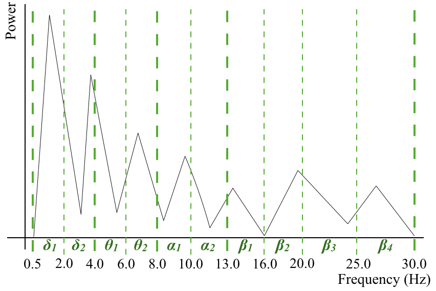
10個に帯域を分けてます.
今回のパラメタ推定の詳しい狙いなどは,以下の奮闘記に書いています.
「最小二乗法によるパラメータ同定奮闘記2」
Pythonプログラムについて
こちらがプログラムになります.
公開してますが,他のユーザが使用するのを意識してないので雑です.
素人が組んだプログラムなので素人には読めると思います(笑)
(できないよりは回れば良いと思っている派なので勘弁ください,,,)
クラスとかそういうオブジェクト指向たっぷりの組み方もいつか勉強しておきます.
1 2 3 4 5 6 7 8 9 10 11 12 13 14 15 16 17 18 19 20 21 22 23 24 25 26 27 28 29 30 31 32 33 34 35 36 37 38 39 40 41 42 43 44 45 46 47 48 49 50 51 52 53 54 55 56 57 58 59 60 61 62 63 64 65 66 67 68 69 70 71 72 73 74 75 76 77 78 79 80 81 82 83 84 85 86 87 88 89 90 91 92 93 94 95 96 97 98 99 100 101 102 103 104 105 106 107 108 109 110 111 112 113 114 115 116 117 118 119 120 121 122 123 124 125 126 127 128 129 130 131 132 133 134 135 136 137 138 139 140 141 142 143 144 145 146 147 148 149 150 151 152 153 154 155 156 157 158 159 160 161 162 163 164 165 166 167 168 169 170 171 172 173 174 175 176 177 178 179 180 181 182 183 184 185 186 187 188 189 190 191 192 193 194 195 196 197 198 199 200 201 202 203 204 205 206 207 208 209 210 211 212 213 214 215 216 217 218 219 220 221 222 223 224 225 226 227 228 229 230 231 232 233 234 235 236 237 238 239 240 241 242 243 244 245 246 247 248 249 250 251 252 253 254 255 256 257 258 259 260 261 262 263 264 265 266 267 268 269 270 271 272 273 274 275 276 277 278 279 280 281 282 283 284 285 286 287 288 289 290 291 292 293 294 295 296 297 298 299 300 301 302 303 304 305 306 307 308 309 310 311 312 313 314 315 316 317 318 319 320 321 322 323 324 325 326 327 328 329 330 331 332 333 334 335 336 337 338 339 340 341 342 343 344 345 346 347 348 349 350 351 352 353 354 355 356 357 | # -*- coding: utf-8 -*- import csv import scipy.signal as sps from scipy.optimize import leastsq import numpy as np import matplotlib.pyplot as plt import matplotlib.animation as animation import matplotlib.patches as patches from time import sleep frame = 241 #定数宣言 N = 512 # サンプル数 dt = 0.002 # サンプリング間隔 p_max = 30.0 p_min = 0.5 #p_band = 1.00000 delta_bound, theta_min, theta_bound, alpha_min, alpha_bound, beta_min, beta_bound1, beta_bound2, beta_bound3 = 2.0, 4.0, 6.0, 8.0, 10.0, 13.0, 16.0, 20.0, 25.0 #ファイル名宣言 inputData = 'exp.txt' outputPara = 'parameters_b_100mass.txt' outputIFFT = 'ifft_b_100mass.txt' outputMovie = 'result_b.mp4' rowN = 2 #配列用意 x_exp = list() x_ifft = np.empty((2,0)) t = list() xd = list() xdd = list() w = list() p = list() x_ifft_s = list() x_exp_s = list() t_s = list() Result = list() F2 = list() freq = list() timecount = 1 #global #const. t_max = 250 t_min = 0 window = N*dt timestep = 0 #timestep def det_band(frequencies): global p_min, p_max, delta_bound, theta_min, theta_bound, alpha_min, alpha_bound, beta_min, beta_bound1, beta_bound2, beta_bound3 f_max = list() f_min = list() k = 0 for frequency in frequencies: if((p_min <= frequency)&(frequency < delta_bound)): f_min.append(p_min) f_max.append(delta_bound) elif((delta_bound <= frequency)&(frequency < theta_min)): f_min.append(delta_bound) f_max.append(theta_min) elif((theta_min <= frequency)&(frequency < theta_bound)): f_min.append(theta_min) f_max.append(theta_bound) elif((theta_bound <= frequency)&(frequency < alpha_min)): f_min.append(theta_bound) f_max.append(alpha_min) elif((alpha_min <= frequency)&(frequency < alpha_bound)): f_min.append(alpha_min) f_max.append(alpha_bound) elif((alpha_bound <= frequency)&(frequency < beta_min)): f_min.append(alpha_bound) f_max.append(beta_min) elif((beta_min <= frequency)&(frequency < beta_bound1)): f_min.append(beta_min) f_max.append(beta_bound1) elif((beta_bound1 <= frequency)&(frequency < beta_bound2)): f_min.append(beta_bound1) f_max.append(beta_bound2) elif((beta_bound2 <= frequency)&(frequency < beta_bound3)): f_min.append(beta_bound2) f_max.append(beta_bound3) elif((beta_bound3 <= frequency)&(frequency <= p_max)): f_min.append(beta_bound3) f_max.append(p_max) f_mix = zip(f_min, f_max) f_mix = sorted(f_mix) f_min, f_max =zip(*f_mix) return f_max, f_min #fft_peak検出用関数 def fft_peak(): global t_s, x_exp_s, x_ifft_s, x_ifft, w, p, F2, freq peak_idx = list() # データのパラメータ freq = np.linspace(0, 1.0/dt, N) # 周波数軸 # 高速フーリエ変換 F = np.fft.fft(x_exp_s) Power = F.copy() # 振幅スペクトルを計算 Power = np.abs(Power) # 振幅を元の信号のスケールに揃える Power = Power / (N/2) # 交流成分はデータ数で割って2倍する Power[0] = Power[0] / 2 # 直流成分 F2 = F.copy() # FFTデータからピークを自動検出 peak_idx = sps.argrelmax(Power, order=1)[0] # ピーク(極大値)のインデックス取得 # ピーク検出感度調整もどき、後半側(ナイキスト超)と閾値より小さい振幅ピークを除外 peak_cut = 0.1 # ピーク閾値 peak_idx = peak_idx[(Power[peak_idx] > peak_cut) & (peak_idx >= p_min) & (peak_idx <= p_max)] selected_peakPower = zip(Power[peak_idx], freq[peak_idx]) peak = sorted(selected_peakPower, reverse=True) p, f = zip(*peak) p = list(p) f =list(f) del f[2:] # print(f) # del p[2:] # print(p) p_max2, p_min2 = det_band(f) if p_min2[0] == p_min2[1]: #ローパスフィルタ&&ハイパスフィルタ F2[(freq > p_max2[0])|(freq < p_min2[0])] = 0.0 elif p_min2[1] == p_max2[0]: #パスフィルタ F2[(freq > p_max2[1])|(freq < p_min2[0])] = 0.0 else: #パスフィルタ F2[(freq > p_max2[1]) | ((freq > p_max2[0])&(freq < p_min2[1])) |(freq < p_min2[0])] = 0.0 # p_max2 = f[0] + p_band # p_min2 = f[0] - p_band # del p[2:] # w = 2.0 * np.pi * f w = f w = [i*2.0*np.pi for i in w] #逆高速フーリエ変換 x_ifft_s = np.fft.ifft(F2) #実数部を取得し、振幅を元のスケールに戻す x_ifft_s = np.real(x_ifft_s)*2 x_ifft_s = np.array(x_ifft_s) t_s = np.array(t_s) x_ifft_m = np.array([t_s, x_ifft_s]) x_ifft = np.c_[x_ifft, x_ifft_m] # 振幅スペクトルを計算 F2 = np.abs(F2) # # 振幅を元の信号のスケールに揃える # F2 = F2 / (N/2) # 交流成分はデータ数で割って2倍する # F2[0] = F2[0] / 2 # 直流成分 #xd と xddの計算 def cal(): global t_s, x_ifft_s j = 0 xd.append(float((x_ifft_s[j+1] - x_ifft_s[j])/dt)) #xd[0] j+=1 for j in range(N-1): xd.append(float((x_ifft_s[j+1] - x_ifft_s[j])/dt))#xd[1] xdd.append(float((xd[j] - xd[j-1])/dt))#xdd[0] t_s = t_s.tolist() x_ifft_s = x_ifft_s.tolist() t_s.pop() x_ifft_s.pop() xd.pop() def func3(param, t_s, x_ifft_s, xd, xdd): global w residual = xdd + (param[0]*xd + param[1]*x_ifft_s + param[2]*x_ifft_s*x_ifft_s*x_ifft_s - param[3]*np.cos(w[0]*t_s)- param[4]*np.sin(w[0]*t_s) - param[5]*np.cos(w[1]*t_s)- param[6]*np.sin(w[1]*t_s)) return residual def lsm(): global t_s, x_ifft_s, xd, xdd para = [0., 0., 0., 0., 0., 0., 0.] #para = [0, 0, 0, 0] t_s = np.array(t_s) x_ifft_s = np.array(x_ifft_s) xd = np.array(xd) xdd = np.array(xdd) params = leastsq(func3, para, args=(t_s, x_ifft_s, xd, xdd)) return params #main関数 def input_Data(): global x_exp, t, rowN with open(inputData, 'r') as InputFile: reader = csv.reader(InputFile, delimiter='\t') for row in reader: t.append(float(row[0])) x_exp.append(float(row[rowN])) # print(x_exp) # print(t) # print(len(x_exp)) # print(len(t)) def main(TimeStep): global x_exp, x_ifft, t, w, p, x_ifft_s, x_exp_s, t_s, xd, xdd, Result i = 0 # for i in range(int(len(x_exp)/N)): xd = list() xdd = list() # for i in range(len(x_exp)/N): x_exp_s = x_exp[TimeStep*N:(TimeStep+1)*N] t_s = t[TimeStep*N:(TimeStep+1)*N] # print(i*N) fft_peak() # print(w) cal() Result = lsm() OutputFile1.write("{:.3f}\t{:.6f}\t{:.6f}\t{:.6f}\t{:.6f}\t{:.6f}\t{:.6f}\t{:.6f}\t{:.6f}\t{:.6f}\n".format(0.510+TimeStep*dt*N,Result[0][0],Result[0][1],Result[0][2],Result[0][3],Result[0][4],w[0],Result[0][5],Result[0][6],w[1])) print("xdd + {:.6f}xd + {:.6f}x + {:.6f}x*x*x - {:.6f}cos{:.6f}t - {:.6f}sin{:.6f}t - {:.6f}cos{:.6f}t - {:.6f}sin{:.6f}t\n".format(Result[0][0],Result[0][1],Result[0][2],Result[0][3],w[0],Result[0][4],w[0],Result[0][5],w[1],Result[0][6],w[1])) return Result #グラフの用意 fig = plt.figure(figsize=(18,16)) ax1 = plt.subplot2grid((5,3), (0,0), colspan=3) ax2 = plt.subplot2grid((5,3), (1,0), colspan=3) ax3 = plt.subplot2grid((5,3), (2,0)) ax4 = plt.subplot2grid((5,3), (3,0), sharex = ax3) ax5 = plt.subplot2grid((5,3), (4,0), sharex = ax3) ax6 = plt.subplot2grid((5,3), (2,1)) ax7 = plt.subplot2grid((5,3), (3,1), sharex = ax6) ax8 = plt.subplot2grid((5,3), (4,1), sharex = ax6) ax9 = plt.subplot2grid((5,3), (2,2)) ax10 = plt.subplot2grid((5,3), (3,2), sharex = ax9) ax11 = plt.subplot2grid((5,3), (4,2), sharex = ax9) #fig.tight_layout() #グラフの初期化 def update_fig(): ax3.cla() ax4.cla() ax5.cla() ax6.cla() ax7.cla() ax8.cla() ax9.cla() ax10.cla() ax11.cla() ax3.set_ylabel('A') ax3.set_ylim(-100, 20) ax3.set_xlim(t_min, t_max) ax4.set_ylabel('B') ax4.set_ylim(-1000, 10000) ax5.set_ylabel('C') ax5.set_ylim(-20, 20) ax6.set_ylabel('omega1 (rad/sec)') ax6.set_ylim(0, 30) ax6.set_xlim(t_min, t_max) ax7.set_ylabel('P1_1') ax7.set_ylim(-20000, 20000) ax8.set_ylabel('P2_1') ax8.set_ylim(-20000, 20000) ax9.set_ylabel('omega2 (rad/sec)') ax9.set_ylim(0, 30) ax9.set_xlim(t_min, t_max) ax10.set_ylabel('P1_2') ax10.set_ylim(-20000, 20000) ax11.set_ylabel('P2_2') ax11.set_ylim(-20000, 20000) def update_fig1(): ax1.cla() ax1.set_title('EPIA') ax1.set_xlim(t_min, t_max) ax1.set_ylabel('EEG (μV)') ax1.set_ylim([-600,600]) ax1.set_xlabel('Time (s)') ax1.plot(t, x_exp, 'k') #時間配列, 実験値配列, 色 def update_fig2(): global t, F2 ax2.cla() ax2.set_ylabel('Power') ax2.set_xlim(0, 50) ax2.set_ylim(0,2000) ax2.set_xlabel('Frequency (Hz)') ax2.plot(freq, F2, 'c') # ax2.plot(freq_exp, fft_exp, 'c') input_Data() OutputFile1 = open(outputPara, mode='w') update_fig1() update_fig2() update_fig() def update(timestep): global timecount, x_ifft result = main(timestep) #描画 #グラフタイトルセット update_fig1() #データプロット r = patches.Rectangle(xy=((timestep-1/2)*window, -600.0), width=window*2, height=1200.0, ec='r', fc='r') ax1.add_patch(r) update_fig2() ax3.plot(timestep*window+window/2, result[0][0], 'r', marker="x", markersize=2) ax3.tick_params(labelbottom="off") ax4.plot(timestep*window+window/2, result[0][1], 'r', marker="x", markersize=2) ax4.tick_params(labelbottom="off") ax5.plot(timestep*window+window/2, result[0][2], 'r', marker="x", markersize=2) ax5.tick_params(labelbottom="off") ax6.plot(timestep*window+window/2, w[0]/(2.0*np.pi), 'b', marker="x", markersize=2) ax6.tick_params(labelbottom="off") ax7.plot(timestep*window+window/2, result[0][3], 'r', marker="x", markersize=2) # ax6.bar(timestep*window+window/2, result[0][3], ec='r') # ax6.bar(timestep*window+window/2, result[0][4], ec='b', bottom=result[0][3]) ax7.tick_params(labelbottom="off") ax8.plot(timestep*window+window/2, result[0][4], 'r', marker="x", markersize=2) ax8.tick_params(labelbottom="off") ax9.plot(timestep*window+window/2, w[1]/(2.0*np.pi), 'b', marker="x", markersize=2) ax9.tick_params(labelbottom="off") ax10.plot(timestep*window+window/2, result[0][5], 'r', marker="x", markersize=2) ax10.tick_params(labelbottom="off") ax11.plot(timestep*window+window/2, result[0][6], 'r', marker="x", markersize=2) ax11.tick_params(labelbottom="off") if timestep+1==frame: update_fig() ani = animation.FuncAnimation(fig, update, interval=50, frames=frame) ani.save(outputMovie) #保存 #plt.show() OutputFile1.close() OutputFile2 = open(outputIFFT, mode='w') writer = csv.writer(OutputFile2, lineterminator='\n', delimiter='\t') x_ifft = x_ifft.T writer.writerows(x_ifft) OutputFile2.close() |
やりたいことが無くなって時間が余ったら見やすいコードに修正します.
アニメーションの意義
理系大学生ならば,発表資料等で,「解析方法」や「実験結果」を説明すると思います.
やはりその時には,動きのある資料の方が良かったりする場合が多いと思います.
価値の高い素敵な発表も,難しすぎて聴衆に理解されないままだと悔しいので,出来る限り納得させる工夫ができたら良いですね.
ブログに公開するのを了承してくださる方で,そういったご相談があれば,一緒に考えますよ〜!
Twitterの方にDM下さい.
では〜!


ダイナミクスの減衰パラメータ”A”が負値(負減衰?)になっている場合があるように見受けられますが,
同定されたパラメータで,生波形と同じ初期値を与えた場合,有限の振幅の波形になるのでしょうか?
宜しくお願いします.